We are now going to see how reaction barrier changes when we solve the reactants in water. Since water is a polar solvent we can anticipate that there will be an effect of some sort. In this part we first create and equilibrate a simulation box with the reactants and water molecules. Then we perform a Linear Transit calculation, using the reaction coordinate of the previous step (figure 3).
QM/MM subdivision
The system consists of the two reactant molecules solvated in water
and one Na+ ion. The ion compensates the overall charge of -1 on the
aliphatc tail (-R, figure 1)). This
system is way too big to be treated at the QM level. Therefore we
divide the system in a small QM part and a much bigger MM part. The QM
part consists of the reactants, without the aliphatic tail and is
described again at the semi-empirical PM3 level, while the
remainder is modelled with the GROMOS96 forcefield. Figure 6 shows the
subdivision used in this part of the tutorial.
In this part of the tutorial we are going to perform again a Linear
Transit calculation, but this time, the reactants are fully
solvated. The details on how to perform a QM/MM Linear transit
calculations in gromacs were discussed previously.
We will again make use of scripts to perform the Linear Transit.
The create_tops.scr and the run.scr script are identical to the ones
we used before, but the get_energies.scr script is slightly
different. In vacuum we could simple take the total potential
energy. In the water, and later in the protein, we don't want to know
the potential energy of the complete system, but rather the internal
energy of the reactans plus the contributions from the interaction of
the reactants with the surroundings. So what we want is
E(reactants)+E(reactant-solvent)+E(reactants-NA+).
localhost:~>mkdir LTwater
localhost:~>mkdir up localhost:~>mkdir down
localhost:~>cd up localhost:~>../create_tops.scr 0.15 0.4 200
localhost:~>../run.scr 0.15 0.4 200
This will take a while, depending on the speed of your computer
system.
localhost:~>../get_ener.scr 0.15
0.4 200 > eqmmm.xvg
localhost:~>cd ../down
execute the create_tops.scr scripts again to
create 51 subdirectories (called step_0, ..., step_50) and create a
topol_A.itp with different constraints lengths in the range 0.15 to
0.12 nm.
localhost:~>../create_tops.scr 0.15 0.12 50
localhost:~>../run.scr 0.15 0.12 50
This will also take a while.
localhost:~>../get_ener.scr 0.15
0.12 50 > eqmmm.xvg
localhost:~>xmgr down/eqmmm.xvg up/eqmmm.xvg
localhost:~>editconf -f
confout.gro -o confout.pdb
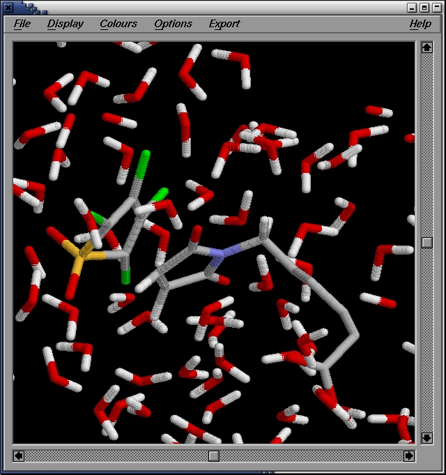
We then use rasmol to visualize the structure:
localhost:~>rasmol confout.pdb
We show the first shell of water.
Clearly there are many water molecules interacting with the molecule.
The minima are at 0.335 nm (-1202.4 kJ/mol) and 0.15125 nm
(-1271.7 kJ/mol) and correspond to the reactant and product states
respectively.
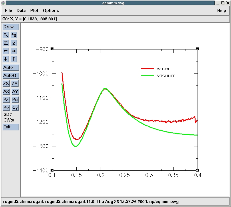
Now, we plot the energy curve we obtained previously for the reaction
in vacuo in the same figure to see the effect of the water on
the energetics of the reaction. We modify a bit the offset of the
vacuum curve to make the comparison easier.
Water is destabilizing the reactants relative to the product and
transition state, making it energetically easier for the reactants to
reach the transition state and form product. However, the reactants
first have to find each other, and then stay together long enough for
reaching the transition state. This is an entropic effect which can be
estimated by different techniques. We will not do that here, as it is
outside the scope of this tutorial.
We have now found the geometries and energies of the transition state,
the reactant state and the prodcut state of the Diels-Alder
cycloaddition in water. Table 3 lists the QM/MM energies of these
geomtries.
Figure 6. Division of the system in a QM
subsystem and an MM subsystem. The QM subsystem is described at the
semi-empirical QM level,
while the remainder of the system,
consisting of the reactants' aliphatic tail, the water molecules and
the Na+ ion, is modeled with the GROMOS96
forcefield.
Finding product, reactant and transition state geometries in
water, using Linear Transit
The starting structure for this calculation is the transition-state
analogue form the x-ray model, we have modified in the previous part of this tutorial. Then we
place this structure in the center of a periodic box and fill that box
with 2601 SPC water molecules and 1 Na+ ion. The total system is
equilibrated, before the Linear transit computation is performed. As
before we will skip this tedious procedure, which has nothing to do
with QM/MM, and use the results instead (confin.gro). The steps we took in the
equilibration process are described here.
#include ions.itp
A complete topology file should look like this topol.top, which is available for
download.
#include flex_spc.itp
The maximum is at 0.20875 nm (-1062.9 kJ/mol). This corresponds to
point 47 in the up subdirectory. Let's have a look at that
structure. We simply go into the directory up/step_47 and use editconf
to convert the confout.gro into confout.pdb 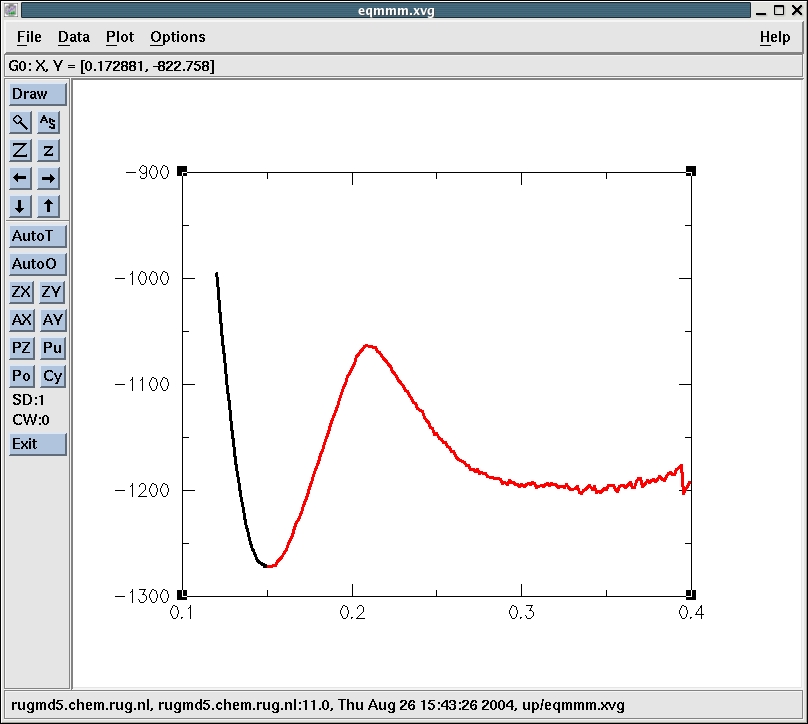
Conclusions
Table 3. Energies of the reactant,
transition state and product geom-
etries in water at the
PM3/GROMOS96 QM/MM level.
The last column lists the energy
differences with respect to the
reactant state.
E (kJ/mol) ΔE (kJ/mol) Reactant -1202.4 0.0
Trans. St. -1062.9 139.5
Product -1271.7 -69.3