With a good guess of what the transition state should look like, it
was rather straightforward to find the transition state geometry. We
will now use the more systematic Linear Transit approach to do the
same.
In the Linear Transit a coordinate is choosen along which the
reactants are transformed into product. This so called reaction
coordinate is varied linearly while all other degrees of freedom are
minimized. Choosing such reaction coordinate requires some intuition
and understanding of the process studied, but is in general easier to
chose than a reasonable guess geometry. The concept of the reaction
coordinate is best explained by an example. In case of a Diels-Alder
cyclo-addition, a good reaction coordinate would be the distance
between the two atom pairs that are forming the two new bonds upon
reaction (figure 3).
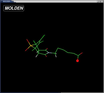
Here we will use the gromacs QM/MM features to perform a Linear
Transit calculation of the Diels-Alder cyclo-addition reaction (figure 1). The -R group, which was
missing in the x-ray model and ignored in the previous part of the
tutorial, will now be taken into account. Because this group is
unlikely to have a large effect on the reaction, we will describe it
at the MM level in our model.
QM/MM subdivision
Figure 4 shows how we split up our system in a QM and MM part. The QM
part consists of the same atoms we were using in the previous vacuum
calculations and is described at the semi-empirical PM3 level
of theory. The remainder of the system, consisting of the tail part
(-R, figure 1) is modeled with the GROMOS96 forcefield.
The QM/MM division splits the systems along a chemical
bond. Therefore, we need to cap the QM subsystem with a so-called link
atom (la, figure 4). This link atom is present as a hydrogen atom in
the QM calculation step. It is not physically present in the MM
subsystem, but the forces on it, that are computed in the QM step, are
distributed over the two atoms of the bond. The bondlength itself is
constrained during the computations.
To make use of the QM/MM functionality in Gromacs, we have to
We also need to know how to do a Linear-Transit in Gromacs:
adding link atoms
At the bond that connects the QM and MM subsystems we introduce a link
atom. In Gromacs we make use of a special atomtype, called LA. This
atomtype is treated as a hydrogen atom in the QM calculation, and as a
dummy atom in the forcefield calculation. The link atoms, if any, are
part of the system, but have no interaction with any other atom,
except that the QM force working on it is distributed over the two
atoms of the bond. In the topology the link atom (LA), therefore, is
defined as a dummy atom:
specifying the QM atoms
Once we have decided which atoms should be treated by a QM method, we
add these atoms, including the link atoms, if any, to the index
file. We can either use the make_ndx program, or hack the atoms into
the index.ndx file ourselves. The index file we will use in this
tutorial is found here: index.ndx. It
is possible to constrain the bonds in the QM subsystem along. It is
also possible not to constrain them, while the bonds in the MM
subsystem are. This is essential for instance if the QM atoms are
supposed to undergo bond-breaking/formation reactions. In this case,
Gromacs' bondtype 5 is used for the bonds in the QM subsystem:
specifying the QM/MM simulation parameters
The last thing we need to do to setup gromacs for performing QM/MM
calculations is to specify what level of QM theory gromacs has to use
for the QM subsystem, what QM/MM interface to use, what multiplicity
the QM subsystem has, and so on. All these things are defined in the
mdp file. The following option lines need to be included for a QM/MM
run:
setting up a Linear-Transit calculation
In this paragraph we describe how to do linear transits with
gromacs. Note that Linear Transist calculations have nothing to do
with QM/MM and can be done with an MM only description as well. We
will refer to the reaction coordinate defined in figure 3.
We want to constrain the distance between the centers of the atompairs
involved in the reaction and minimize all other degrees of freedom in
the system. The way we can impose our constraint in gromacs, is to put
a dummy atom (atomtype XX), with no interaction whatsoever with any
other atom of the system, exactly in the middle of the atompairs
(figure 3) and constrain the dummy-dummy distance.
The dummy is constructed every step of the simulation/optimization, so
that it is always exaclty in the middle between the atompair. Note, in
the current version of gromacs, constraints between dummies are not
allowed yet, so we will use a little trick here. The trick is
explained here. For now, it is not important to
know the details of this trick. Furthermore, already in the next
release of gromacs it will be possible to apply the dummy-dummy
constraints we need here.
performing a Linear-Transit calculation
Now that we know how to constrain the reaction coordinate, we are
going to perform minimizations at different constraint lengths. We
create different subdirectories, one for every Linear-Transit
point. We perform the minimizations in these subdirectories and use
the result as input for the minimization in the next
subdirectory. After all minimizations along the reaction coordinate
have been done, we collect the energies from the subdirectories and
plot them as a function of the reaction coordinate.
The procedure is straightforward, but tedious. Therefore, we will make
use of scripts. With the first script we create the subdirectories and
place the topology files with different constraint legths in them. The
second script then goes into the subdirs one by one, runs grompp en
mdrun. Finally a third script runs g_energy, which retrieves the
energies from the outputfile ener.edr and collects the energies as a
function of the constraint lenght. The scripts are available for
download:
The usage of all three scripts is: scriptname.scr dist1 dist2 steps where dist1 and
dist2 are the first and last points along the reaction coordinate
respectively and steps is the number of points we want to have on the
reaction coordinate.
Using these scripts we are going to perform a Linear Transit
calculation on the Diels-Alder reaction in figure 1 in vacuo, along the
reaction coordinate shown in figure 3.
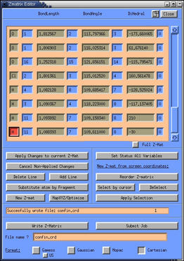
localhost:~>molden -P analogue.pdb
localhost:~>mkdir LTvacuo
localhost:~>./create_tops.scr 0.12 0.5 200
localhost:~>./run.scr 0.12 0.5 200
This will take a while, depending on the speed of your computer
system.
localhost:~>./get_ener.scr 0.12 0.5 200 >
eqmmm.xvg
localhost:~>xmgr eqmmm.xvg
localhost:~>editconf -f confout.gro -o confout.pdb
We then use rasmol to visualize the structure:
localhost:~>rasmol confout.pdb
It looks verly much like the one we optimized in the previous
step. You can check if it is a TS by perfoming a frequencies
caclulaiton on this structure, using gaussian, just like we did before.
The minima are at 0.4468 nm (-342.826kJ/mol) and 0.1485 (-388.276
kJ/mol) and correspond to the reactant and product state respectively,
and are shown here, along with the transition state again.
We have now found the geometries and energies of the transition state,
the reactant state and the prodcut state of the Diels-Alder
cycloaddition in vacuo. Table 2 lists the potential energies of
these geomtries. A direct comparison with the energies and energy
differences found using the optimization routines of gaussian98 (tabel 1) in not valid, because in the
current computations the aliphatic tail (-R, figure 1) was taken into account
explicitly, while it was ignored in the previous computations.
Figure 3. Suitable Reaction Coordinate for a
Diels-Alder reaction. The distance (d) between the centers of the atom
pairs involved in the cyclo-
Once the reaction coordinate is choosen, we slowly progress along that
coordinate, while minimizing all other degrees of freedom. In
practice, the reaction coordinate is constrained or restrained at a
number of distances. Afterwards, the potential energy is plotted as a
function the reaction coordinate. The maximum of this curve is the
transition state and the minima are the reactant and product
states.
addition is restrained or constrained,
while all other degrees of freedom are minimized.
Figure 4. Division of the system in a QM
subsystem and an MM subsystem. The QM subsystem is described at the
semi-empirical QM level,
while the remainder of the system,
consisting of the reactants-aliphatic tail is modeled with the
GROMOS96 forcefield.
[ dummies2 ]
Note, a link atom has no mass.
LA QMatom MMatom 1 0.65
Furthermore, the bond itself is replaced by a constraint:
[ constraints ]
Note that, because in our system the QM/MM bond is a carbon-carbon
bond (0.153 nm), we use a constraint length of 0.153 nm, and dummy
position of 0.65. The latter is the ratio between the ideal C-H bondlength
and the ideal C-C bond length. With this ratio, the link atom is always 0.1 nm
away from the
QMatom, consistent with the carbon-hydrogen bondlength. If
the QM and MM subsystems are connected by a different kind of bond, a
different constraint and a different dummy position, appropriate for
that bond type, are required. The QM/MM topology file for the
reactants shown in figure 4 is found here: topol_A.itp.
QMatom MMatom 2 0.153
[ bonds ]
QMatom1 QMatom2 5
QMatom2 QMatom3 5
QMMM = yes
Note that the default options are shown here. The actual options
depend on the system. The mdp file we will use for the QM/MM
computations in vacuo is located here: LT.mdp. In case one choses as the
QMmethod a semi-empirical method, such as AM1 or PM3, the
QMbasis is ignored.
QMMM-grps = QMatoms
QMmethod = RHF
QMbasis = 3-21G*
QMMMscheme = ONIOM
QMcharge = 0
QMmult = 1
[ dummies2 ]
where 1.6 is the current constraint length.
dummy1 atom1 atom2 1 0.5
dummy2 atom3 atom4 1 0.5
[ constraints ]
dummy1 dummy2 2 1.6
Finding product, reactant and transition state geometries in
vacuo, using Linear Transit
The maximum is at 0.2093 nm (-149.924 kJ/mol). This corresponds to
point 47. Let's have a look at that structure. We simply go into the
directory step_47 and use editconf to convert the confout.gro into
confout.pdb 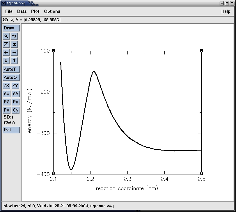
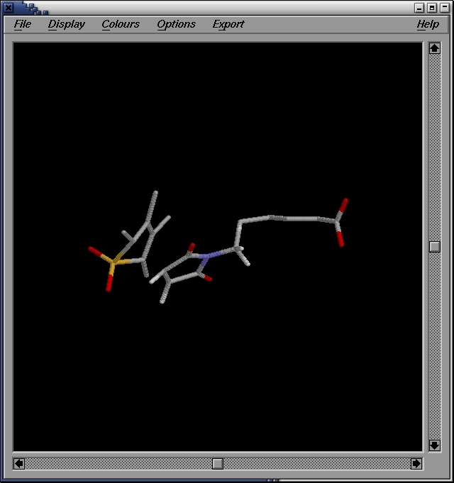
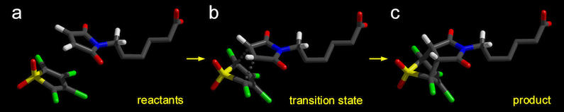
Figure 5. Reactant (a), Transition State (b),
and Product (c) geometries in vacuo, found with the Linear
Transit method. The
energies of these structures are listed in table
2.
Conclusions