We have seen that in water the energy of the transition state is lower that in vacuo, with respect to the reactants. Now we will calculate the energy curve in the protein to see the effect of the protein environment on the reaction.
QM/MM subdivision
The fully solvated protein system is too large for even a
semi-empirical QM calculation. Therefore, we resort to a QM/MM
description of the system. The way we split up the system in a small
QM part and a much bigger MM part, is shown in figure 7. The QM part
consists of the same atoms as before and is again described at the
semi-empirical PM3 level of theory. The remainder of the
system, consisting of the tail part (-R, figure 1) of the reactants, the
protein, the water molecules and the chloride ions, is modeled with
the GROMOS96 forcefield.
In this part of the tutorial we are going to perform a third Linear
Transit calculation, but this time, the reactants are fully solvated.
With the QM/MM subdivision shown in figure 7, we will perform the
third and last Linear Transit computation. The details of how to
perform such a calculation in gromacs can be reviewed here.
The starting structure for this calculation is the x-ray model of the
1CE catalytic antibody by Xu et al.. Remember that in the x-ray
model, the -R group of the analogue was not resolved. So we need to
add it ourselves. We take the modified transition-state analogue of part II of this tutorial and fit it onto
the analogue in the x-ray model. After the fit, we minimize the tail
part, keeping the rest of the protein fixed.
Then we place this modified protein model in a periodic box, fill that
box with water and equilibrate the water. Subsequently, we add 6 Cl-
ions to compensate the overall net charge of -6 on the protein and
equilibrate again. The procedure of preparing the system for the QM/MM
geometry optimization is straightforward, but
time-consuming. Therefore, we skip fitting and equilibrating and use
the result (confin.gro) instead. An
outline of the preparation is avalaible here.
And here are the scripts we use this time to perform the Linear
Transit:
localhost:~>mkdir LTprotein localhost:~>cd LTprotein
localhost:~>mkdir up localhost:~>mkdir down
localhost:~>cd up localhost:~>../create_tops.scr 0.15 0.4 200
localhost:~>../run.scr 0.15 0.4 200
This will take a while, depending on the speed of your computer
system.
localhost:~>../get_ener.scr 0.12 0.4 200 > eqmmm.xvg
localhost:~>cd ../down
and execute the create_tops.scr scripts again to create 51
subdirectories (called step_0, ..., step_50) and create a topol_A.itp
with different constraints lengths in the range 0.15 to 0.12 nm.
localhost:~>../create_tops.scr 0.15 0.12 50
localhost:~>../run.scr 0.15 0.12 50
This will take a while again.
localhost:~>../get_ener.scr 0.15 0.12 50 > eqmmm.xvg
localhost:~>xmgr up/eqmmm.xvg down/eqmmm.xvg
localhost:~>editconf -f
confout.gro -o confout.pdb
We then use rasmol to visualize the structure:
localhost:~>rasmol confout.pdb
We zoom a bit in on the active site, showing interacting residues and
water molecules:
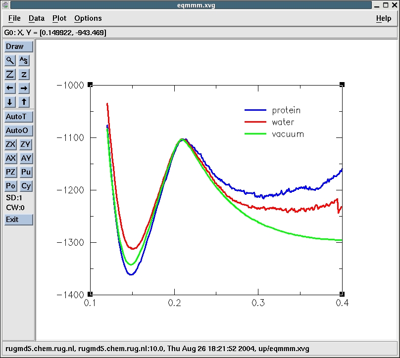
The minima are at 0.306250 nm (-1216.4 kJ/mol) and 0.15 nm
(-1360.8 kJ/mol) and correspond to the reactant and product states
respectively. Figure 8 shows the reactant, transition and product
states of the system.
Now, we plot the energy curves in vacuo, water and te protein all in
the same figure. We manipulate the offsets of the curves to make the
comparison easier.
The protein is is stabilizing the transition state relative to
reactants even more that the water. The reaction rate therefore should
be highest in the protein. Note however that alse here the entropic
contribution is not included. The reactants need to be bound by the
protein first to form the reactive protein-substrate complex. These
steps can be studied with different simulation techniques.
We have now found the geometries and energies of the transition state,
the reactant state and the prodcut state of the Diels-Alder
cycloaddition in the active site of the catalytic Diels-Alderase
antibody. Table 4 lists the total QM/MM energies of these geomtries.
Figure 7. Division of the system in a QM
subsystem and an MM subsystem. The QM subsystem is described at the
semi-empirical QM level,
while the remainder of the system,
consisting of the reactants-aliphatic tail, protein, water molecules
and ions is modeled with the GROMOS96
forcefield.
Finding product, reactant and transition state geometries in the
fully solvated protein
Note we will not use the topol_A.itp, but instead create a new one
with a different constraint length for the reaction coordinate for
every point of the Linear Transit.
The maximum is at 0.21 nm (-1102.9 kJ/mol). This corresponds
to point 48 in the up subdirectory. Let's have a look at that
structure. We simply go into the directory up/step_48 and use editconf
to convert the confout.gro into confout.pdb 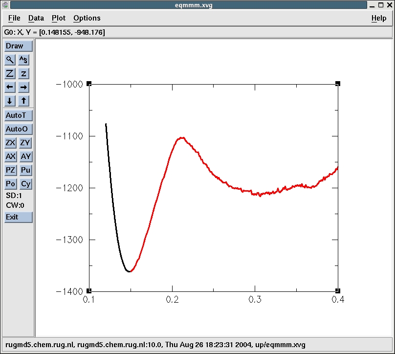
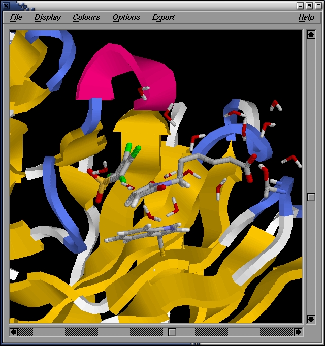
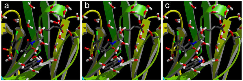
Figure 8. Reactant (a), Transition State (b)
and Product (c) geometries in the active site of the catalytic
antibody, found with the Linear
Transit method. The energies of these
structures are listed in table 4.
Conclusions
Table 4. Energies of the reactant,
transition state and product geom-
etries in the solvated protein
at the
PM3/GROMOS96 QM/MM level.
The last column lists the
energy
differences with respect to the
reactant state.
E (kJ/mol) ΔE (kJ/mol) Reactant -1216.4 0.0
Trans. St. -1102.9 113.5
Product -1360.8 -144.4